Activation functions

Before we move onto training our neural network, it is important to learn about activation functions.

Activation functions are functions that determine whether your ‘neurons’ will fire or not depending on your dot product calculation is similar to neurotransmitters.

Hint

Activation functions are best visually represented. If you struggle with visualizing graphs in your head, or don’t know the maths behind these functions, it is best you watch sentdex’s video on this topic.

Firstly, let’s get key terms down.

• Input - the input (in terms of activation function) refers to the dot product calculation.
• Output - depending on the function, this refers to the dot product calculation that has been modified by the function.

So, why is linearity flawed?

If we were to just use weights and biases, our neural network’s activation function would be linear:

$y=mx+c$ where $m$ is your weight and $c$ is your bias value. Essentially, whatever the input is, all output values will follow a simple linear line based on the weight and bias. And if the output affects the rest of the neural network, that means the network will fit on this linear line.

Now, imagine if you’re given complex data where somethings may be right and other things may be wrong - and your neural network has to learn it. In a way, it has to “bend” this line so that it can learn the things that are right and prune the things that are wrong. If it doesn’t bend, then how does it account for those differences in input?

This is why linearity is flawed. Non-linearity activation functions fix this issue.

The vanishing gradient

The vanishing gradient refers to the issue where a neural network struggles to learn and adapt.

When you get derivative of an activation function, you can map where a function is activated and deactivated. However, if a function flattens, the gradient of that line is getting closer and closer to 0.

This means that even if the input size is insanely out of proportion, the model won’t know the difference between that and if it’s only slightly wrong - making it hard to learn.

This is usually tied to backpropagation and the activation function’s derivative, which is important for training.

Common activation functions

Rectified Linear Unit (ReLU)

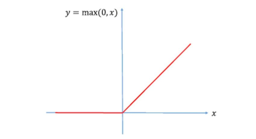
ReLU is a piecewise linear function that is extremely simple and easy to compute. It has the following properties:

$f(x)=\{\begin{array}{l}x\le 0:0\\ x>0:x\end{array}$

1. For inputs of 0 or less than 0, the output is set to the 0.
2. For inputs of anything greater than 0, then the output is set to the input.

You can control where a neuron activates or deactivates, affecting the graph, by changing the weights and biases so that it’s negative when unused and positive when used. This way, you can can manipulate the output so that the network can properly learn and predict.

Pros	Cons
Fast and easy to compute	Harder for the model train as it reduces “how wrong” into 0s.
Simple to visualize	Hard to account the model cannot make a prediction (all 0s).

See sentdex’s video at 12:27 to see how this ReLU function can fit itself into a sine wave.

Code

class activation_ReLU:
    def forward(self, inputs):
        self.outputs = np.maximum(0, inputs)

It’s extremely simple - it clamps all data between the minimum of 0 and the input. This means the the value, at minimum, is 0.

before activation:
[[0.11627268, 0.00841107, 0.08436441, 0.21167282],
[0.41092453, -0.03484579, 0.2306009, 0.3395143]]

after activation:
[[0.11627268, 0.00841107, 0.08436441, 0.21167282],
[0.41092453, 0, 0.2306009, 0.3395143]]

as you can see from above, the negative value before has turned into 0 as per the ReLU function.

import numpy as np
np.random.seed(0)
inputs = [[0.2, 0.5, 1.2],
            [1.2, 1.1, 0.6]]
            
weights = [[1.0, 0.5, 1.3],
            [2.0, 3.2, -0.8]]
bias = [1.0, 1.2]
 
 
class neural_layer:
    def __init__(self, weights, bias):
        self.weights = weights
        self.bias = bias
        
    @staticmethod
    def new(input_size, output_size):
        # input_size = number of neurons in the previous layer that provide an input to the current layer
        # output_size = number of neurons outputted to the next layer
        weights = 0.1 * np.random.randn(input_size, output_size)
        return neural_layer(weights, np.zeros((1, output_size)))
        
    def forward(self, inputs):
        self.outputs = np.dot(inputs, self.weights) + self.bias
 
class activation_ReLU:
    def forward(self, inputs):
        self.outputs = np.maximum(0, inputs)
 
  
 
layer1 = neural_layer.new(3, 4)
layer1.forward(inputs)
 
activation1 = activation_ReLU()
activation1.forward(layer1.outputs)
 
print(activation1.outputs)

Sigmoid

v7labs.com

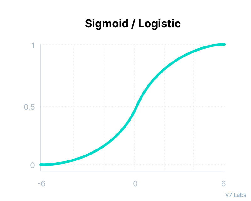
The sigmoid is a function that evens out and infinitely approaches 1 or 0. Unlike the ReLU function, negative values don’t output a 0.

$f(x)=\frac{1}{(1+e^{-x})}$

Properties of the sigmoid function:

1. The larger or smaller the input data, it becomes infinitely closer to 1 or 0 respectively, flattening out.
2. It outputs between the range of 0 and 1 - making it useful for binary computation (2 possible choices) and probability.

Pros	Cons
Smooth gradient to prevent random jumps in output.	Prone to gradient vanishing because the gradient is extremely close to 0.
Differentiable for backpropagation.	Exponential calculations are more expensive.

Code

class activation_sigmoid:
    def forward(self, inputs):
        self.outputs = 1/(1+np.exp(-inputs))

Softmax Function

botpenguin

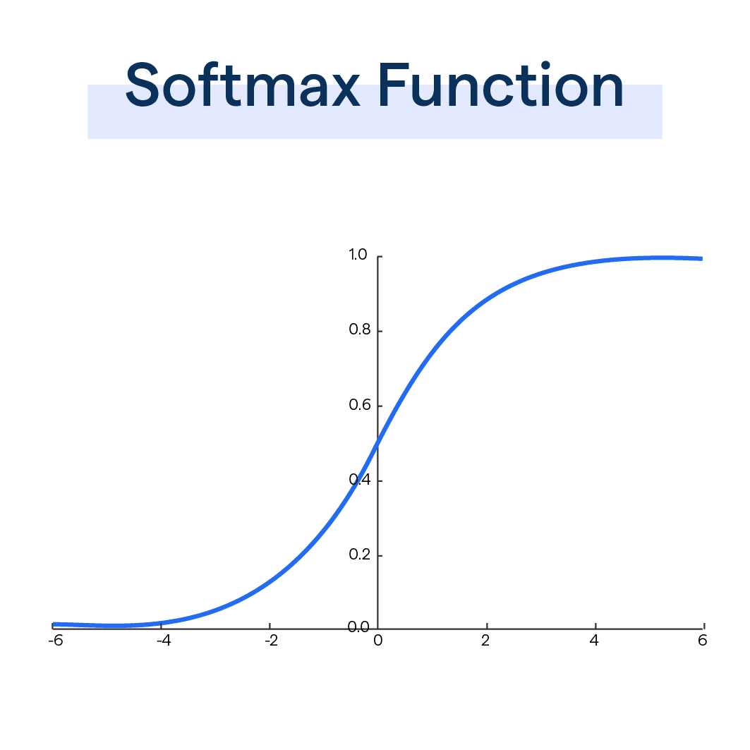
The softmax function is similar to sigmoid, but rather than outputting a single probability, the softmax function outputs the probability distribution across all neurons (classes) each output representing the neuron’s probability that sums up to a 1.

$\sigma (\vec{z})=\frac{e^{z_i}}{{\Sigma }_{j=1}^K{e}^{z_j}}$

$\vec{z}$ = the input vector

$e^{z_i}$ = standard exponential function for input vector

$K$ = number of classes (neurons) in the multi-class classifier (results)

$e^{z_j}$ = standard exponential function of output vector

Now, that looks really confusing… but I promise it’s not.

1. Given a vector of inputs, usually called scores or logits, you calculate the exponents with $e^{z_i}$ for each element in the vector. Find the sum of these exponents, this will form the denominator.
2. For each element in the vector, find the exponent again ($e^{z_i}$). This is your numerator.
3. Calculate the division for every element. This will give you the probability of each input. This process is called normalization.

Because of softmax’s ability to produced multiclass probability statements, is differentiable and more, it is the reason why the softmax function is usually found in the output layer.

Code

class activation_softmax:
	def forward(self, inputs):
		exponents = np.exp(inputs - max(inputs))
		self.outputs = exponents / exponents.sum(axis=-1, keepdims=1)

To explain the code:

• We get the list of exponents with np.exp(), which applies the exponential function to every element of the np.array.
  • However, exponentials grow quickly; values can quickly become too large to be handled, causing overflow. To combat this, you can just subtract inputs by the max(inputs),
• we then set the outputs of the class to the exponents, divided by the sum (which we use exponents.sum() method that’s built into np.arrays). The .sum() method takes in 2 parameters:
  • axis = -1: this means that the sum will always be calculated by the sum of values of the rows, not columns.
  • keepdims=1: this means that the dimensions (size) of the array is kept in the result. This is especially important if you have different batches of data that you are processing.